When to Use Descriptive Statistic in Research
Descriptive Statistics – Definition
Descriptive statistics is a branch of statistics that aims at describing a number of features of data usually involved in a study. The main purpose of descriptive statistics is to provide a brief summary of the samples and the measures done on a particular study. Coupled with a number of graphics analysis, descriptive statistics form a major component of almost all quantitative data analysis.
Descriptive statistics are quite different from inferential statistics. Basically, descriptive statistics is about describing what the data you have shown. For inferential statistics, you are trying to come up with a conclusion drawing from the data you have.
For example, we can use inferential statistics to try and give an indication of what the population thinks from the sample. We can also use inferential statistics to judge on the probability of something occurring based on the behavior of the sample of data taken for a study.
Thus, inferential statistics are used mainly to infer based on the sample data we have at hand to make conclusions. On the other hand, descriptive statistics is used mainly to give a description of the behavior of the sample data.
Descriptive statistics are usually used in presenting a quantitative analysis of data in a simple way. In a study, there are quite a number of variables that are usually measured. Therefore, descriptive statistics comes in to break this numerous amounts of data into a simple form.
For example, one might be interested to find the average passes a footballer makes in a single match. Clearly, there are quite a number of activities in a single game; therefore we can use descriptive statistics to make this simpler. Here we can get a single number that will help us describe very many discrete events. Another instance is determining the how a student performs in school.
Usually, we use the Grade Point Average. This is just a single number that gives a general indication of the performance of a single individual. The moment one looks at the GPA of a student, he can tell the potential of that student on the various courses that he/she takes.
It is important to note that, when using a single value to describe a large set of data, there is a possibility that you are going to change the original meaning of the data or lose some important detail. This is because; the number just gives an overall impression of the aspects but does not provide the exact detail of the same.
For example, the GPA of a student does tell whether the student performed well in the easy subjects and failed the hard one or vice versa. However, regardless of these shortcomings, descriptive statistics are still the best way of summarizing a wide range of data and aid in making comparisons between the same.
Let’s now get an in-depth look at descriptive statistics
Here, we are going to look at the concept of univariate analysis. This is basically the examination of different cases of a single variable at the same time. There are three main areas that we are going to look at:
- The distribution
- The measure of central tendency
- The dispersion
These are the common characteristics that we will want to identify in our variables.
-
The Distribution
The distribution is a summary showing the frequency of single values of the ranges of a variable. A simple distribution table will list all their values against the number of persons or units each of them had. For example, the simplest way of describing the distribution of university student based on their year of study is to list the percentage of students or the number of students in every year. We can also describe the gender of a sample by listing the percentage of males and females or the numbers of each.
In such cases, the variables involved are quite a few such that we are in a position to comfortably list all them and make a quick summary of the numbers involved in each value. But then, there are cases where the number is too large, for example when handling the GPA or income. In such cases, there are quite a number of possibilities in terms of values and all the values will carry a few people. In such cases, the raw scores need to be grouped in terms of a range of values. For example, the raw scores can be grouped in terms of the ranges of a letter grade e.g.
| Raw Score | Grade |
| 100-70 | A |
| 70-60 | B |
| 60-50 | C |
| 50-40 | D |
| 40-0 | E |
We can also use a frequency distribution to describe a single variable. Depending on the variable involved, we may represent all of the values or group them into categories.
For example, when dealing with variables such as price, temperature or age, it may not be reasonable to determine the frequency of each individual value. So in such a case, we group the value into ranges and determine the frequency of each range. The frequency distribution can be shown in form of a table or a graph.
Apart from that, we may also show distributions in terms of percentages. For example, we can use percentages to describe the following:
- Percentage of people in various age groups
- Percentage of people in various income levels
- Percentage of people in various ranges of test scores
-
The measure of Central Tendency
From the term central, the measure of central tendency involves determining the value at the center of a distribution. We have three main measures of central tendency:
- Mean
- Median
- Mode

What is Mean Statistics?
This is the most common method used in the measure of central tendency. It is the average of all the samples involved. To determine the mean of a sample, you only need to find the sum of all the value involved and divide them by the number of the values.
For example, if you want to find the mean of the score of students in a particular test, you need to sum up all the scores and divide them by the number of students. For example, to calculate the mean score of the marks of ten students with the following values involved:
50, 67, 35, 46, 21, 77, 92, 46, 88, 63
The sum = 584
Mean = 585/10
= 58.5
What is Median Statistics?
The median statistic is the value found in the exact middle of a set of values. To find the median of a set of values, you will need to organize all the values in a numerical order and identify the value at the center of the sample. For example, if you have 100 values, them the 50th value would be the median. In our case above, the median would be:
First, let’s arrange them in ascending order:
21, 35, 46, 46, 50, 63, 67, 77, 88, 92
Here we have position 5 and 6 in the middle, therefore, to get the median we are going to interpolate them by adding the two then dividing them by 2.
(50+63)/2= 56.5
What is the Mode Statistic?
In a set of values, the mode is the frequently occurring value. The mode is usually determined by identifying the most occurring number. You will also need to arrange the numbers in an ascending order then count each of them to identify the most frequently occurring.
For our example above, the most occurring number is 46. It occurs two times in the same set of value. We can as well have two modal values in a set of values. An example of this case always happens in bi-modal distribution where there are always two values that occur frequently.
Note that, in the same set of values, we have obtained totally different values for the measures of central tendency:
Mean = 58.5
Median = 56.5
Mode = 46
For a normal distribution, the mean, median and the mode are usually equal.
-
Dispersion
Dispersion is a term used to describe how values have spread around the central tendency. We have to common means of measuring dispersion that is range and standard deviation.
-
Range
The range is just the maximum value minus the minimum value.
For our example above, the highest value is 92 and the lowest is 21. So the range is
=92-21
=71
-
Standard Deviation
This is the most detailed and the most accurate description of dispersion. This is because it shows how the different values in the set, relate to the mean.
Let’s look at our example:
21, 35, 46, 46, 50, 63, 67, 77, 88, 92
To compute the standard deviation, we first need to find the differences between the values and the mean.
21-58.5= -37.5
35-58.5= -23.5
46-58.5= -12.5
46-58.5= -12.5
50-58.5= -8.5
63-58.5= 4.5
67-58.5 = 7.5
77-58.5 = 18.5
88-58.5= 29.5
92-58.5 =33.5
Note that, all the values above the mean have positive discrepancies while the values below the mean have negative ones.
The next step is to square all the discrepancies:
-37.5x-37.5=1406.24
-23.5x-23.5= 552.25
-12.5x-12.5=156.25
-12.5 x-12.5=156.25
-8.5x-8.5=72.25
4.5×4.5=20.25
7.5×7.5=56.25
18.5×18.5= 342.25
29.5×29.5 = 870.25
33.5 x 33.5= 1122.25
Now we need to determine the variance:
We get this by, finding the sum of the squares of the discrepancies (sum of squares) then divide them by (n-1).
Variance = Sum of Squares/ (n-1)
= 4754.49/9
=528.27
Our standard deviation is now the square root of the variance
SQRT (528.27)
=22.98
This computation seems so complicated but it is actually very simple. We can capture it in the formula below.
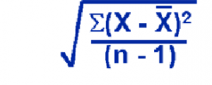
Where:
X= Each Value
¯X = mean
N= number of value
E=summation
The standard deviation can be described as the square root of the sum of the squared deviations from the mean divided by the number of values minus one.
It is important to note that, it is possible to calculate the univariate statistics manually; it can be very tedious especially when dealing with many variables. There are quite a number of statistics software that can help in doing so. An example is SPSS.
The standard deviation is a very important descriptive statistic because it allows us to make a number of conclusions based on the values we have. If we assume that our values are distributed normally or bell-shaped or something close to this, then we can make the following conclusions:
- At least 58% of all the values in the sample are found within one standard deviation of the mean
- At least 95% of the values in the sample are found two standard deviations of the mean
- At least 99% of all the values in the sample fall within three standard deviations of the mean.
Such kind of information is very vital especially when we want to compare the performance of two individual samples based on a single variable. This is possible even in cases when the two variables have been measured in completely different scales.
Read also: “Can I pay someone to write my research paper?” – Yes, you can. Experienced academics will do it for you.
Importance of Descriptive Statistics
Descriptive statistics are very vital because it helps us in presenting data in a manner that can be easily visualized by people. This, therefore means, the data can be easily absorbed by people.
For example, if you are presenting the performance of students in a test, then the measure of central tendency can give an indication of how the class performed.
Useful information: Buying dissertations online has never been easier.
For example, the mode can tell the score that most of the students got. The mean can tell the average performance of the class. On the other hand, the measure of spread can be used to summarize the performance of a group of students. For example, the range can tell the bracket of scores the students got.
In general, descriptive statistics is a great way of breaking raw data into meaningful piece of information that can be easily understood by people they are intended for. However, presenting raw data can be sometimes important because it helps in keeping the original information and the meaning is not distorted.